Examples

Via configuration files

Hello world

We consider the configuration file example1.toml in the examples folder (the animation in the GitHub home page was based on this configuration file). If the results are to be saved in a folder called ‘hello_world’, this is achieved by the following command:

expreccs -i example1.toml -o hello_world

Then we can change in line 25 the BC type for the site from ‘flux’ to ‘pres’, and run the following command to only simulate the site model:

expreccs -i example1_pres.toml -o hello_world -m site

We can do the same to add the pore volumes from the regional reservoir on the site boundaries by setting in line 25 ‘porvproj’:

expreccs -i example1_porvproj.toml -o hello_world -m site

Finally, we consider the case where we add injector/producers on the site boundary, and to also visualize the results in PNGs figures, we run the following command:

expreccs -i example1_wells.toml -o hello_world -m site -p yes

Below are some of the figures generated inside the postprocessing folder:

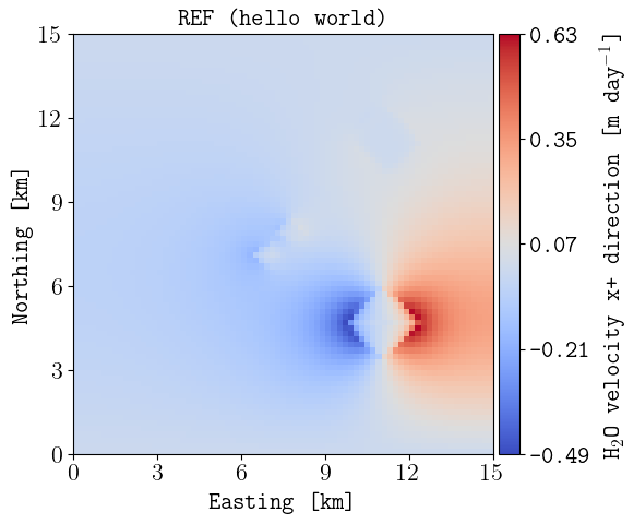
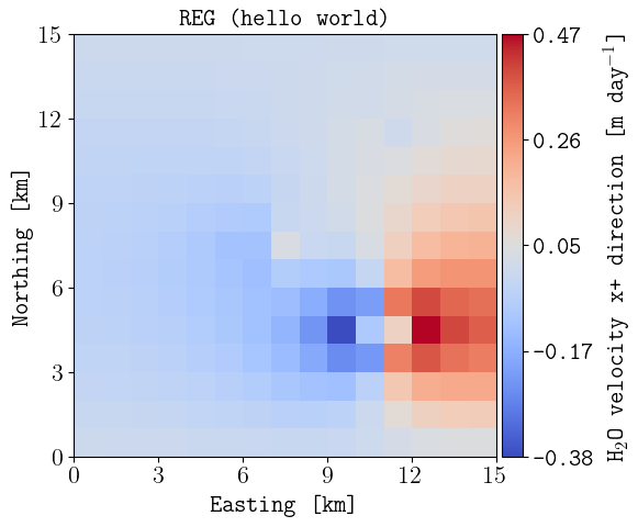
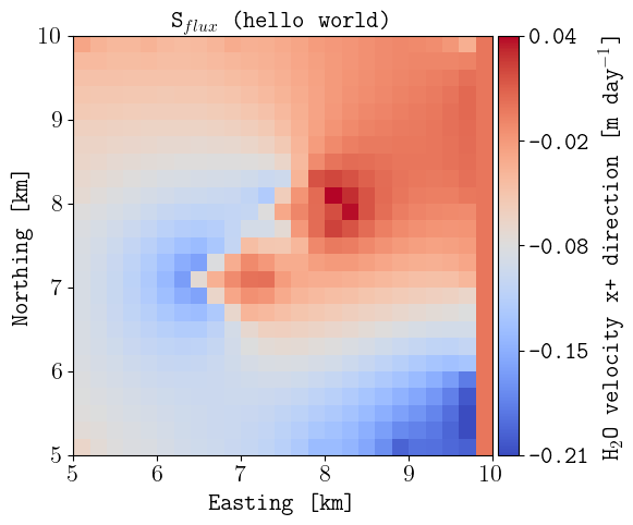
Final water velocity (m/day) in the x direction for (top) the reference, (middle) regional, and (bottom) site (with fluxes as BC). The figure names in the postprocessing folder are hello_world_reference_watfluxi+.png, hello_world_regional_watfluxi+.png, and hello_world_site_flux_watfluxi+.png respectively.

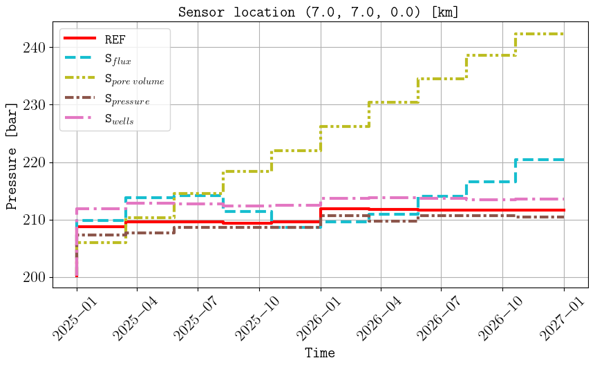
Comparison of cell pressures on the sensor location (top), well BHPs (middle), and minimum distance from the CO2 plume to the site boundaries (bottom). The figure names in the postprocessing folder are hello_world_sensor_pressure_over_time.png, hello_world_summary_BHP_site_reference.png, and hello_world_distance_from_border.png respectively

Layered model

The configuration file example2.toml set a more complex geological model with more grid cells (1 417 500). This was used to generate the animation (using ResInsight) in the introduction section by running

expreccs -i example2.toml -m reference

Tip

This example shows how expreccs can be used to generate the requiered input files to run OPM Flow for heterogenous layered models at different grid sizes, which can be used for further studies such as optimization. Regarding the configuration files in examples/paper_2025, these are explained in this manuscript.

Via OPM Flow decks

Regular boundaries

See/run the test_2_generic_deck.py for an example where expreccs is used in two given models (regional and site, in this case they are created using the expreccs package, but in general can be any given geological models), generating a new input deck where the pressures are projected.

expreccs -i 'path_to_the_regional_model path_to_the_site_model'

For example, to run the test, this can be achieved by executing:

pytest --cov=expreccs --cov-report term-missing tests/test_2_generic_deck.py

To visualize/compare results between the model with static (input) and dynamic (generated by expreccs) boundary conditions, we can use our friend plopm:

plopm -i 'tests/configs/rotate/simulations/site_closed/SITE_CLOSED tests/configs/rotate/simulations/expreccs/EXPRECCS tests/configs/rotate/simulations/reference/REFERENCE' -v sgas -s ',,1 ,,1 ,,1' -subfigs 1,3 -suptitle 0 -cbsfax 0.2,0.95,0.6,0.02 -d 24,8 -cformat .1f -f 20 -xunits km -yunits km -xformat .0f -yformat .0f -x '[0,15000]' -y '[0,15000]' -delax 1

Comparison of the gas saturation on the top cells at the end of the simulations.

Tip

You can install plopm by executing in the terminal:

pip install git+https://github.com/cssr-tools/plopm.git

See also the test_4_site_regional.py, where the two-stage approach is demonstrated in a site and regional deck generated using sandwich.toml. In this test the functionality to select if the bc mappings are written per fipnums, i.e., if there is an offset between the site and regional models along the z direction, then using -z 1 builds the interpolators per corresponding fipnums in the regional and site models. In addition, the flag -e 0 set the interpolators to be defined by pressure increase and not by pressure values. If you run that test, then using plopm:

plopm -i 'tests/regional/REGIONAL tests/expreccs/EXPRECCS tests/expreccs_dpincrease/EXPRECCS_DPINCREASE tests/expreccs_perfipnum/EXPRECCS_PERFIPNUM' -v rpr:3

Comparison of the different functionality to mapp the dynamic boundary conditions. Here, rpr:3 (fipnum equal to 3) corresponds to the top part of the sandwich (three layers with the middel layer inactive) in the regional model, while to the bottom part in the site model.

Non-regular boundaries

The previous examples show the application to sites with reguler boundaries, i.e., prescribed in a rectangle. This example shows how the flag -n 1 can be used to project the pressures in a non-regular boundary. For simplicity, this example does not include wells in the schedule, but you can add wells if you are curious.

We start with a deck with only one cell, then we refined the deck, and after we extract the submodel. To this end, we use another friend: pycopm.

Tip

You can install pycopm by executing in the terminal:

pip install git+https://github.com/cssr-tools/pycopm.git

The terminal commands are the following in the same location as the SIMPLE.DATA deck

pycopm -i SIMPLE.DATA -l R -w REFINED -g 199,319,0
pycopm -i REFINED.DATA -l S -w SUBMODEL -v 'xypolygon [15e3,80e3] [60e3,80e3] [60e3,10e3] [55e3,10e3] [55e3,05e3] [50e3,05e3] [50e3,10e3] [33e3,10e3] [33e3,24e3] [15e3,24e3] [15e3,80e3]' -p 0 -m all

The previous commands generate two decks: REFINED.DATA and SUBMODEL.DATA, where the former one is our regional model and the later one the SITE model. We proceed to run the models:

flow REFINED.DATA
flow SUBMODEL.DATA

Now we can apply expreccs and run the generated model:

expreccs -i "REFINED SUBMODEL" -n 1 -o expreccs
flow expreccs/EXPRECCS.DATA

For the following figure, it is necessary to include in the REGION section of the REFINED.DATA the file “OPERNUM_EXPRECCS.INC” and rerun it. Then, using plopm:

plopm -i 'REFINED expreccs/EXPRECCS' -v opernum -s ',,1 ,,1' -r 0 -xunits km -xlnum 5 -yunits km -yformat .0f -ylnum 5 -xformat .0f -subfigs 1,2 -d 16,12 -cbsfax 0.1,0.95,0.8,0.02 -f 30 -c Set1_r

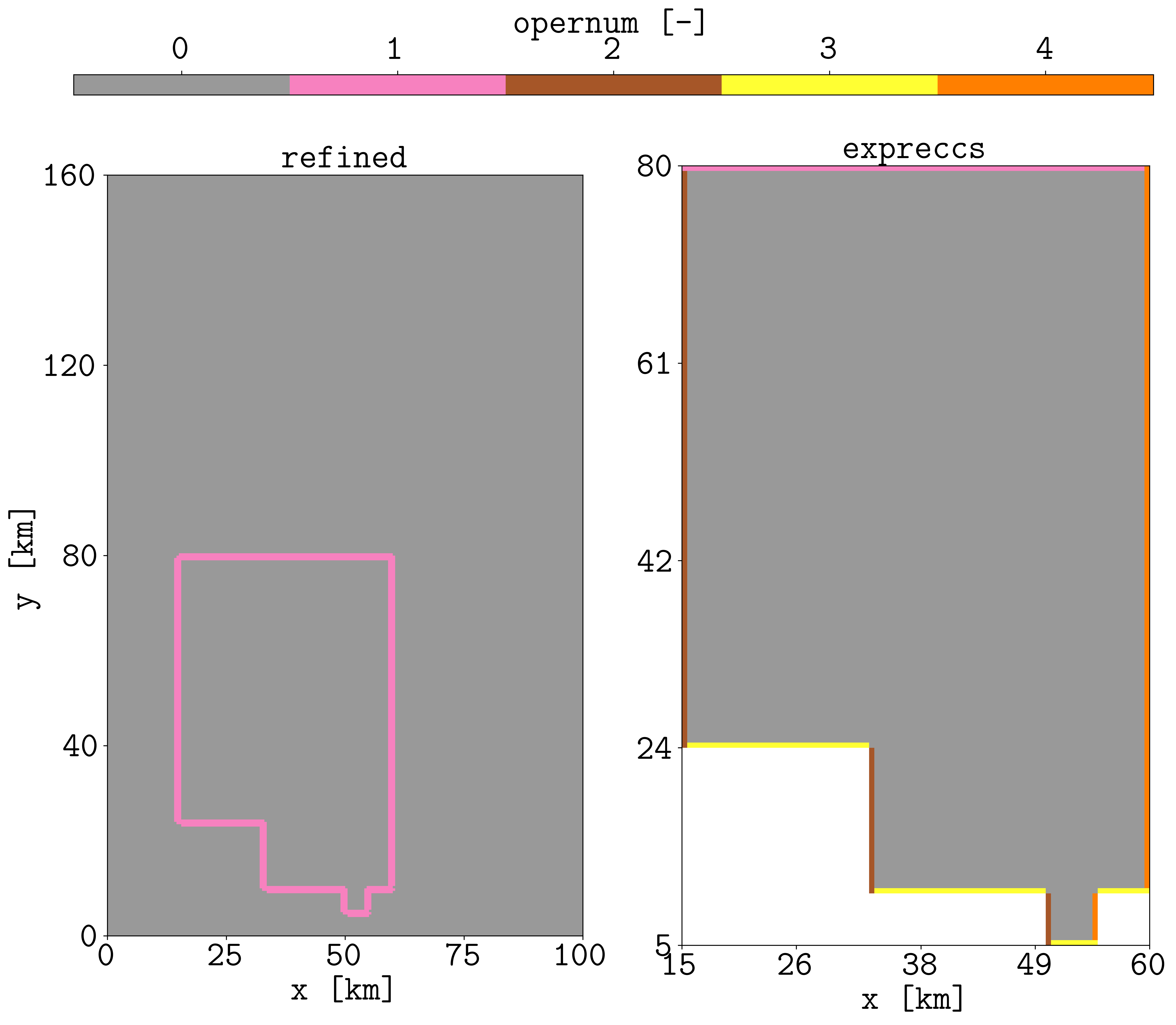
In the regional model (left), expreccs writes the location of the overlapping cells with the site model in the OPERNUM variable, while in the site model this variable is used to label the ij direction of the boundary conditions.