Examples
Image
In this example we consider the micromodel described in the configuration file section.
The image is available in the examples folder in the Github page with the default name ‘microsystem.png’. The configuration file corresponds to the one in the configuration file section and it is saved as ‘parameters.toml’ (the default name for the configuration file). Since ‘image’ is the default entry for the simulation setup, and assuming that the command ‘gmsh’ in the terminal executes Gmsh, then to run the whole framework (meshing, flow, and tracer):
pymm -i microsystem.png -p parameters.toml -t all
The execution time was ca. 20 minutes and the following are screenshots of the simulation results:


Simulation results of the (top) pressure, (middle) velocity, and (bottom) tracer concentration.
Device
Here we consider the same image and configuration file as in the previous example, but we are interested now on the device setup (the flow is from the top-left corner to the bottom-right corner of the device). Then we add the corresponding flag to the pymm executable:
pymm -t all -m device
The execution time was ca. 35 minutes and the following are screenshots of the simulation results:
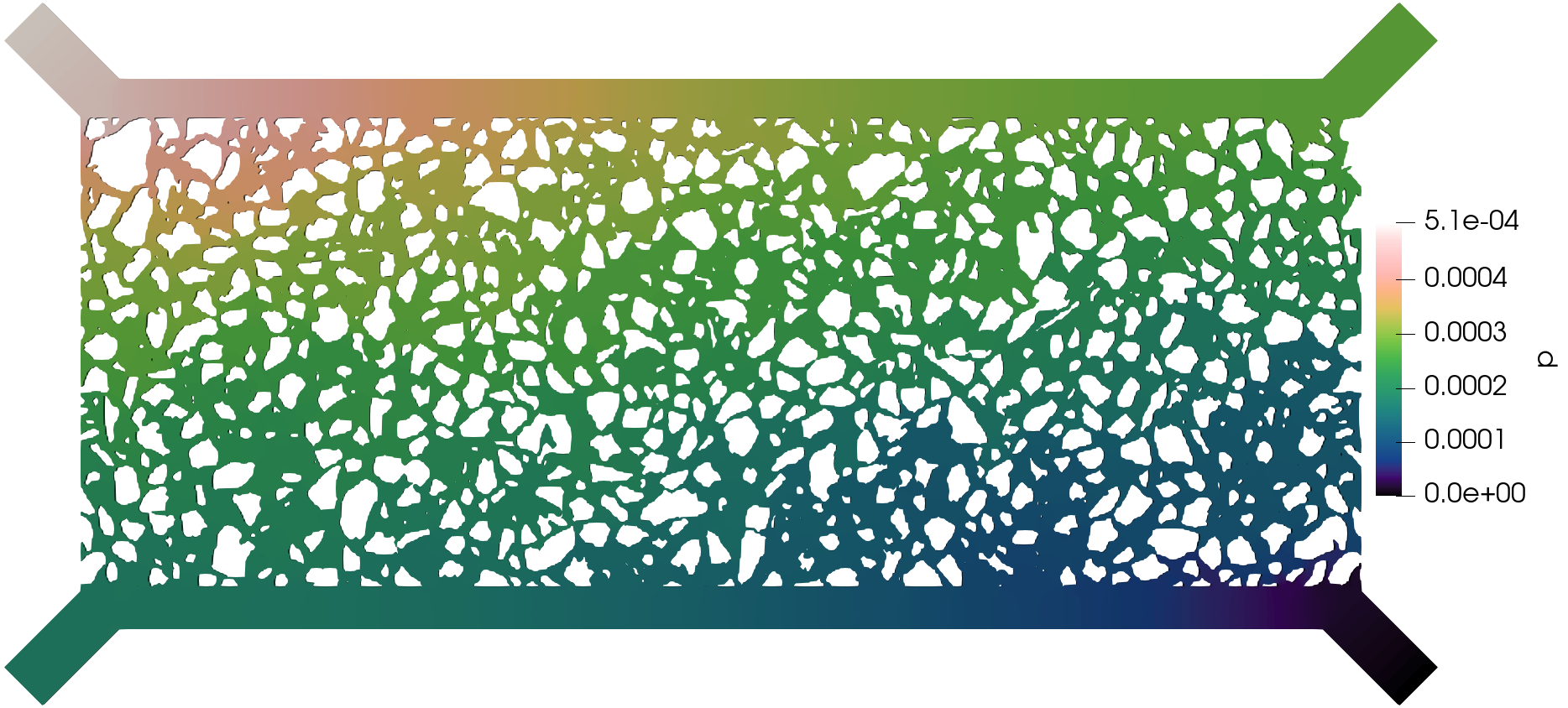
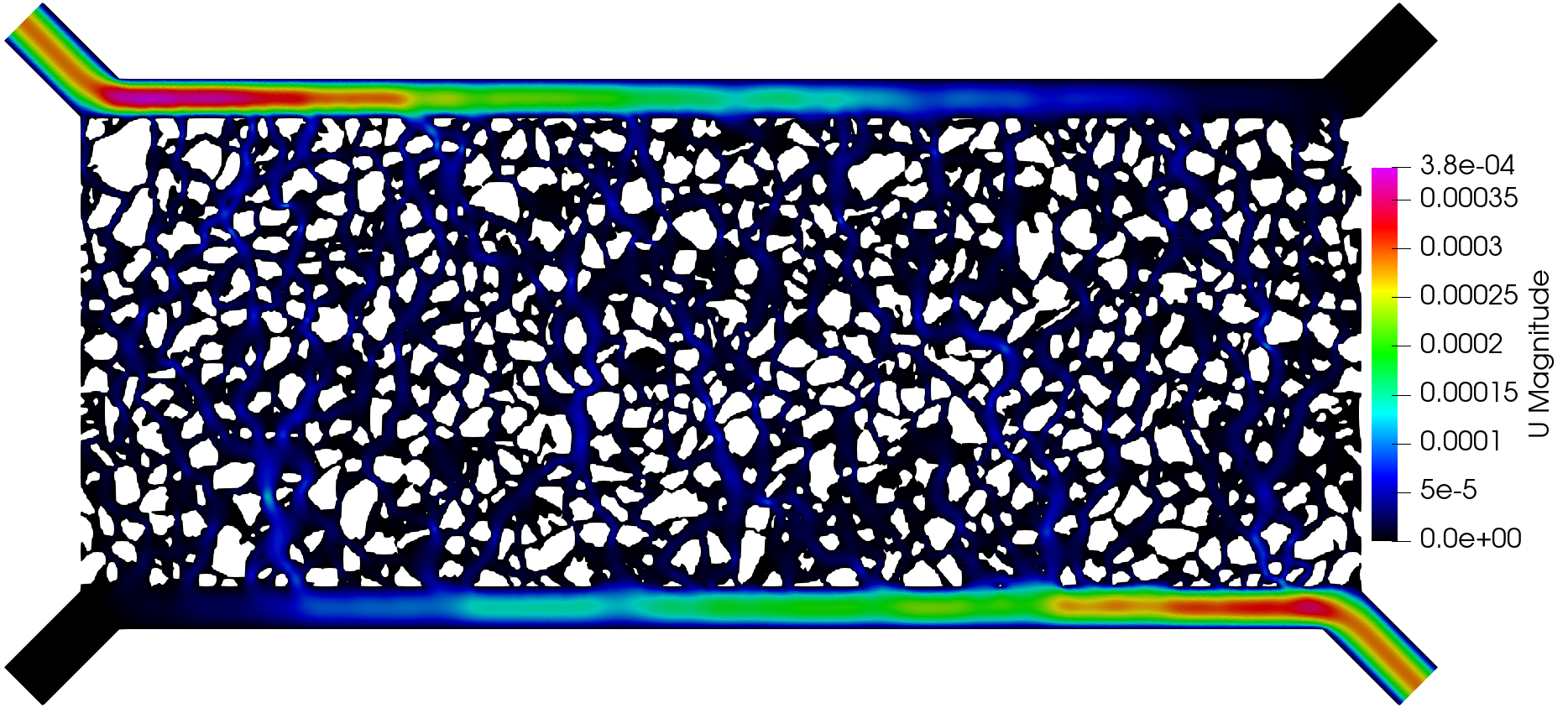
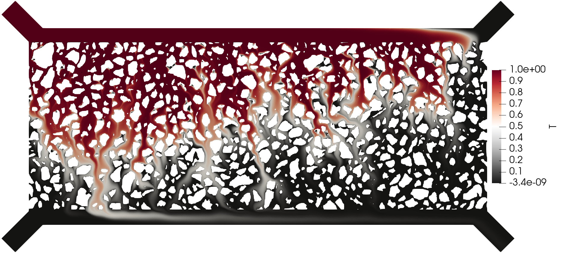
Simulation results of the (top) pressure, (middle) velocity, and (bottom) tracer concentration.
Online
In this example we consider a micromodel available online in Fig. 2a in Joekar-Niasar et al. 2009.
The image was extracted by screenshot and saved with the name ‘online.png’ (1068x1068 pixels). The configuration file was saved as ‘configuration.toml’ and contained the following text:
 1#Set the pymm parameters
 2lenght = 600e-6       #Image-related, length of the microsystem [m]
 3width = 600e-6        #Image-related, height of the microsystem [m]
 4tickness = 1.8e-6     #Image-related, depth of the microsystem [m]
 5grainMeaning = 1      #Image-related, 0 if the grains in the image are light colors (e.g., white) or 1 for dark colors (e.g., black)
 6threshold = 0.5       #Image-related, threshold for converting the image to binary
 7rescale = 1           #Image-related, rescaled factor for the input image
 8grainsSize = 50       #Image-related, minimum size of the grain clusters
 9borderTol = 1         #Image-related, tolerance to approximate the border as polygon
10grainsTol = 1         #Image-related, tolerance to approximate the grains as polygon
11lineWidth = 1         #Figure-related, line width to show the contours in the produced figures
12channelWidth = 6e-6   #Device-related, width of the top and bottom channels in the micromodel device [m]
13meshSize = 1e-6       #Mesh-related, mesh size [m]
14viscocity = 1e-6      #Fluid-related, kinematic viscosity [dynamic viscosity/fluid_density, m2/s]
15diffusion = 1e-12     #Fluid-related, diffusion coefficient for tracer [m2/s]
16inletLocation = "top" #Simulation-related, inlet bc location (left, top, right, or bottom)
17inletValue = 2.0e-3   #Simulation-related, inlet boundary condition (pressure/fluid_density, [Pa/(kg/m3)])
18tracerTime = 120      #Simulation-related, end time for the tracer simulation [s]
19tracerWrite = 1       #Simulation-related, time interval to write the tracer results [s]
20pressureConv = 1e-7   #Solver-related, convergence criterium for the pressure solution in the numerical scheme for the Stokes simulation
21velocityConv = 1e-8   #Solver-related, convergence criterium for the velocity solution in the numerical scheme for the Stokes simulation
22iterationsMax = 10000 #Solver-related, maximum number of iterations for the Stokes simulation in case the convergence criteria have not been reached
23tracerStep = 1        #Solver-related, time step in the numerical scheme for the tracer simulation [s]
Here we used a version of Gmsh built from source, then we gave the path to the executable via the ‘-g’ flag. Since we are interested in the flow and tracer simulations, then we add the flag ‘-t all’. Then, the following command was exectued in the terminal:
pymm -i online.png -p configuration.toml -m device -t all -gmsh /home/AD.NORCERESEARCH.NO/dmar/Github/gmsh/build/gmsh
The execution time was ca. 15 minutes and the following are screenshots of the simulation results:
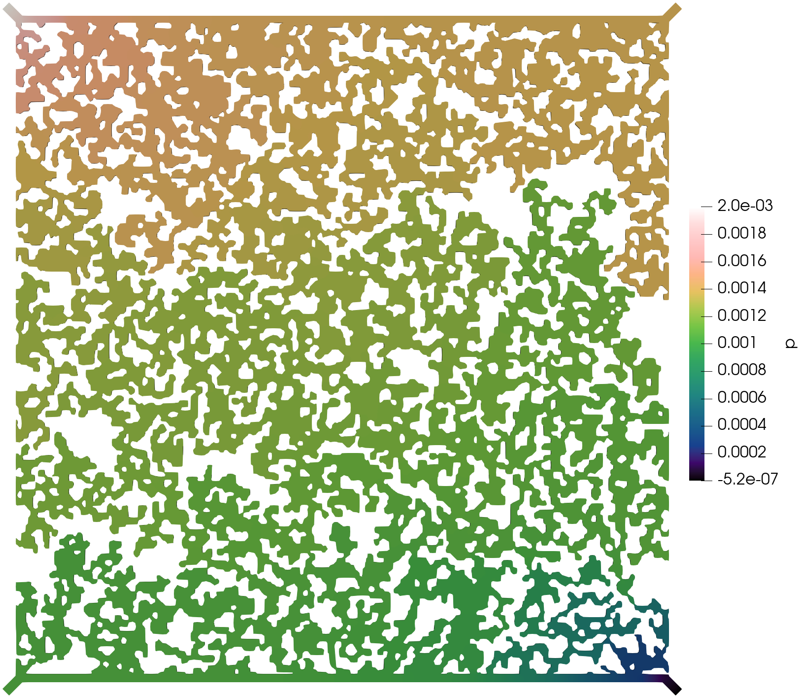
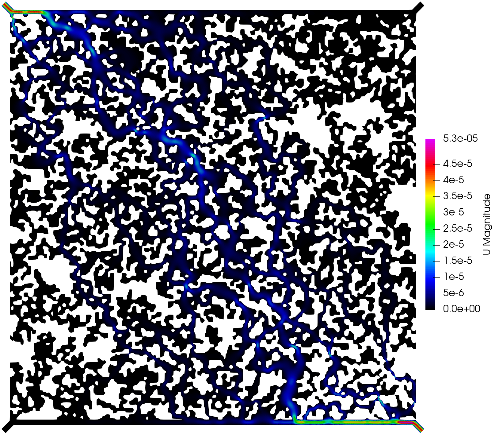
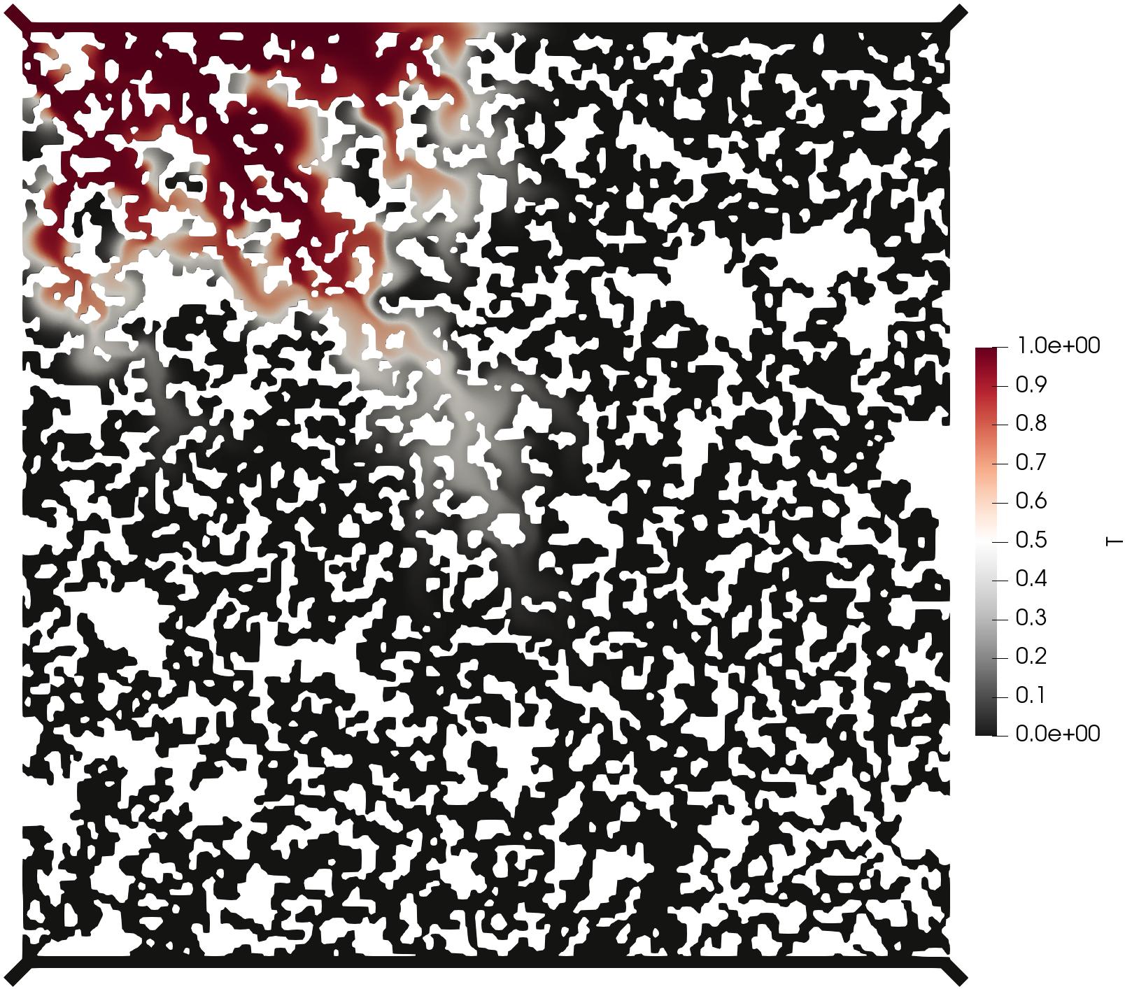
Simulation results of the (top) pressure, (middle) velocity, and (bottom) tracer concentration.