Configuration file

The following configuration file is available in the examples folder in the GitHub repository as co2.toml and in the examples documentation section the simulation results are shown.

The first input parameter in the configuration file is:

#Set mpirun, the full path to the flow executable, and simulator flags (except --output-dir)
flow = "flow --relaxed-max-pv-fraction=0 --enable-opm-rst-file=true --newton-min-iterations=1 --enable-tuning=true"

If flow is not in your path, then write the full path to the executable, as well as adding mpirun if this is supported in your machine (e.g., flow = “mpirun -np 8 /Users/dmar/Github/opm/build/opm-simulators/bin/flow –relaxed-max-pv-fraction=0”).

Reservoir-related parameters

The following input lines are:

#Set the model parameters
model = "co2store" #Model: co2store, co2eor, foam, h2store, or saltprec
template = "base" #Template file (see src/pyopmnearwell/templates/)
grid = "cake" #Grid type: cake, radial, core, cartesian2d, coord2d, tensor2d, cartesian, cpg3d, coord3d, or tensor3d
adim = 60 #Grid cake/radial: theta [degrees]; core: input/output pipe length [m]; cartesian2d, coord2d, tensor2d: width[m]
xdim = 100 #Length [m] (for cartesian/cpg3d/coord3d/tensor3d, Length=Width=2*xdim)
xcn = [80] #Number of x-cells [-]; coordinates for grid type coord2d/coord3d [m]; numbers of x-cells for grid type tensor2d/tensor3d [-]
xfac = 2 #Exponential factor for the telescopic x-gridding (0 to use an equidistant partition)
diameter = 0.1 #Well diameter [m]
pressure = 100 #Pressure [Bar] on the top
temperature = [40,40] #Top and bottom temperatures [C]
initialphase = 0 #Initial phase in the reservoir (0 wetting, 1 non-wetting)
pvmult = 1e10 #Pore volume multiplier on the boundary [-] (-1 to ignore; 0 to use well producers instead)
perforations = [1,5,6] #Activate perforations [-], number of well perforations [-], and length [m]
hysteresis = "Killough" #Add hysteresis (Killough or Carlson, 0 by default, i.e., no hysteresis)
zxy = "2-2*mt.cos((2*mt.pi*x/50)) + 10*(x/100)**2" #The function for the reservoir surface

Here we first select the physical model and the corresponding template. To add additional models (e.g., blackoil), one could look at the opm-tests decks, convert the necessary input decks and files to mako templates, add them to the src/pyopmnearwell/templates folder, and extending the Python scripts in the src/pyopmnearwell/utils folder. In the following line we select type of grid and the second entry defines the length of the inlet/outlet tubes for the core, theta aperture for the radial/cake/coord2d/tensord2d grids, the width of the cells for the cartesian2d grid, or it is ignored for the 3D cartesian grids (the width and number of cells is set equal to the ones in the x directions). See/Run the tests/geometries configuration files for these grids. Then we set the length of the reservoir, as well as the number of grid elements in the x direction (for the y/theta direction we use the ‘adim’ variable with exception to the core/3D grids where the width and number of cells is set equal to the ones in the z/x directions). The xfac entry defines the exponential factor for the telescopic serie used to generate the x partition (if set to 0 then an equidistance partition is generated).

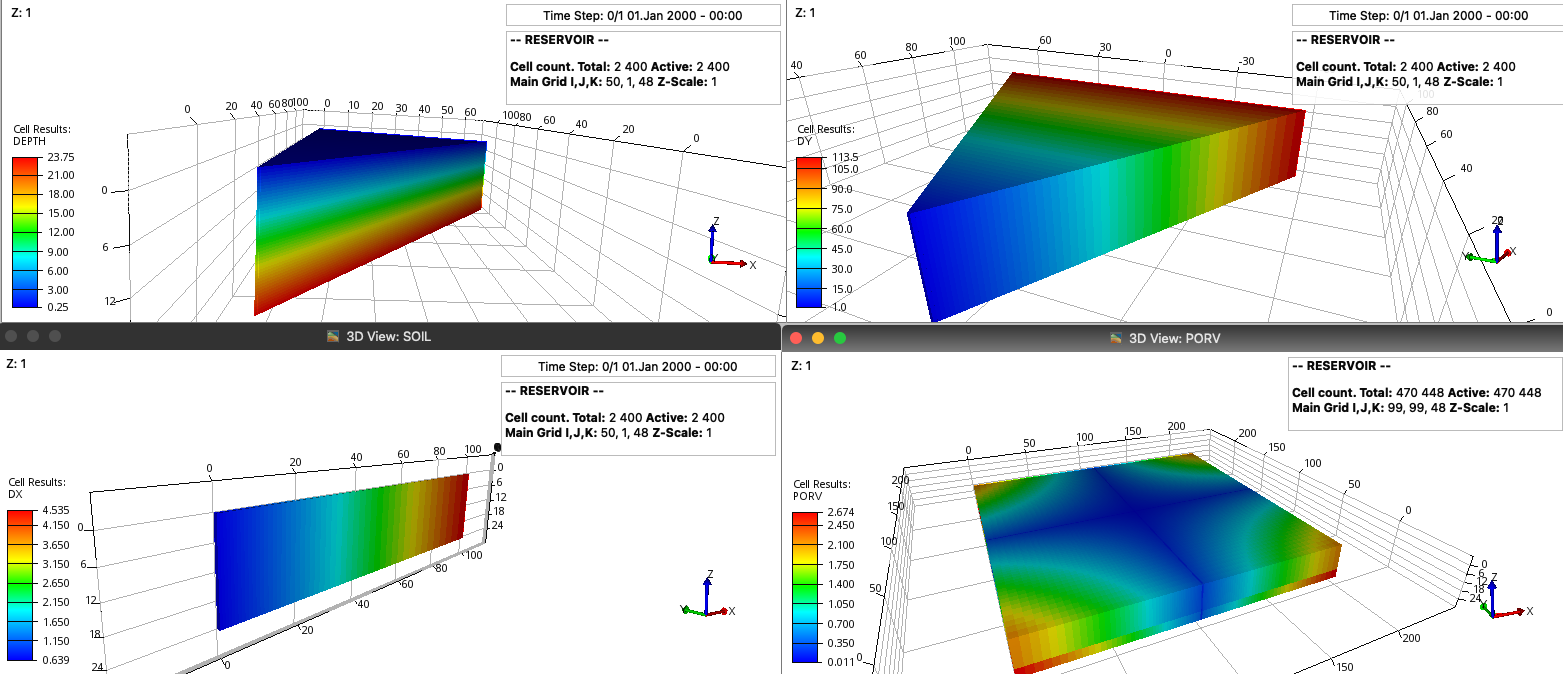
Four different grids by setting the line ‘grid’ and ‘adim’ to ‘radial’ ‘36’ (top left, showing the depth), ‘cake’ ‘60’ (top right, showing the y-direction cell size), ‘cartesian2d’ ‘1’ (bottom left, showing the x-direction cell size), and ‘cartesian’ (bottom right, showing the cell pore volume).

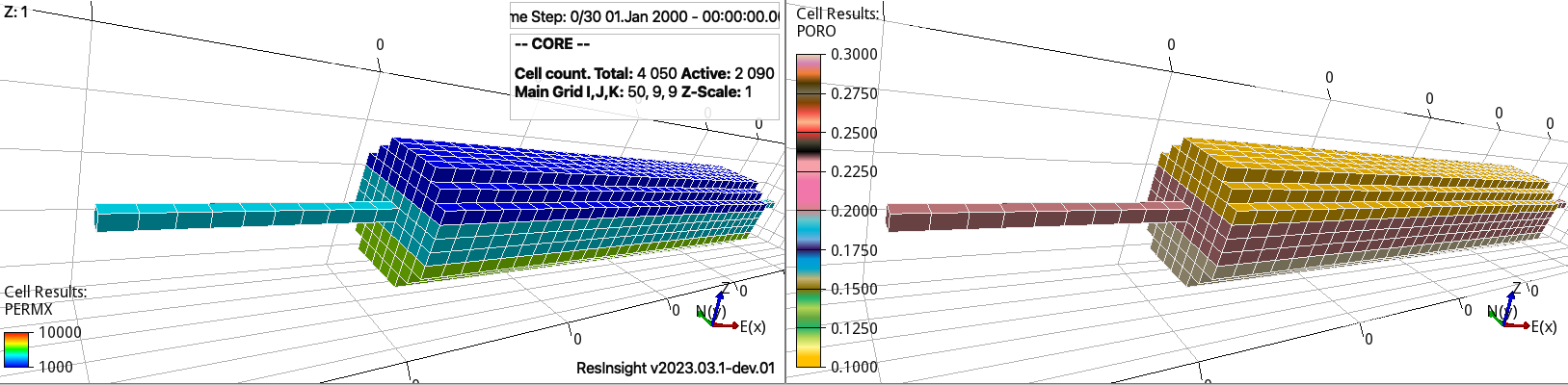
Example of core geometry (generated by running the examples/h2core.toml configuration file).

We then define additional parameters for the reservoir properties, as described in each configuration file.

Rock-related parameters

The following entries define the rock related parameters:

#Set the saturation functions
krw = "krw * ((sw - swi) / (1.0 - sni -swi)) ** nkrw"        #Wetting rel perm saturation function [-]
krn = "krn * ((1.0 - sw - sni) / (1.0 - sni - swi)) ** nkrn" #Non-wetting rel perm saturation function [-]
pcap = "pen * ((sw - swi) / (1.0 - swi)) ** (-(1.0 / npen))" #Capillary pressure saturation function [Bar]

In this example we consider properties for the sands number 2 to 5 as described in the 11th SPE CSP:

#Properties sat functions: 1) swi [-], 2) sni [-], 3) krw [-], 4) krn [-], 5) pen [Bar], 6) nkrw [-], 7) nkrn [-],
#8) npen [-], 9) threshold cP evaluation, 10) ignore swi for cP? (sl* for cplog) (entry per layer, if hysteresis, additional entries per layer)
safu = [[0.14,0.1,1,1,8655e-5,2,2,2,1e-4,0],
[0.12,0.1,1,1,6120e-5,2,2,2,1e-4,0],
[0.12,0.1,1,1,3871e-5,2,2,2,1e-4,0],
[0.12,0.1,1,1,3060e-5,2,2,2,1e-4,0],
[0,0,1,1,0,1,1,1,1e-4,0],
[0.14,0.2,1,1,8655e-5,2,3,2,1e-4,0],
[0.12,0.2,1,1,6120e-5,2,3,2,1e-4,0],
[0.12,0.2,1,1,3871e-5,2,3,2,1e-4,0],
[0.12,0.2,1,1,3060e-5,2,3,2,1e-4,0],
[0,0,1,1,0,1,1,1,1e-4,0]]

Since the ‘activate perforations option’ is set to 1, then we add an extra line after the 4 rock properties to define the ones in the perforations (Line 32). Since the hysteresis option is activated, then the imbibition saturation functions are defined by adding as many additional lines as number of rocks (+1 if the perforations are activated, lines 33 to 37 in this example).

Now for the rock properties:

#Properties rock: 1) Kxy [mD], 2) Kz [mD], 3) phi [-], 4) thickness [m], and 5) no cells in the z dir [-] (entry per layer)
rock = [[101.324,10.1324,0.2,6,6],
[202.650,20.2650,0.2,6,6],
[506.625,50.6625,0.2,6,6],
[1013.25,101.325,0.25,6,6],
[2013.25,201.325,0.45]]

As seen from the previous values, the finnest sand corresponds to the top one and it gets coarser towards the bottom. The last two entries define the z size of the layer and number of cells, while for the perforations these have the thickness of one single cell.

Well-related parameters

Now we proceed to define the schedule for the injection well. Here the injection well is located from the top to the bottom on the left side of the domain and the injection is given as kg/day:

#Define the injection values (entry per change in the schedule):
#1) injection time [d], 2) time step size to write results [d], 3) maximum time step [d]
#4) fluid (0 wetting, 1 non-wetting), 5) injection rates [kg/day]
inj = [[7,1e-1,5e-2,1,57611.52],
[7,1e-1,5e-2,0,57611.52],
[7,1e-1,5e-2,1,57611.52]]

Here CO2 (non-wetting phase) is injected for seven days printing the results 70 times and limmiting the time step to 5e-2 days, after water (wetting phase) is injected for the same period at the same mass rate, and finally CO2 is reinjected for the same period.