Examples

Hello world

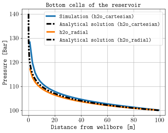
In this example we consider the configuration file ‘h2o.toml’ available in the examples folder (link to the file), where the co2store model is used and only water is injected in a radial grid.

If the generated files are to be saved in a folder called ‘hello_world’, then this is achieved by the following command:

pyopmnearwell -i h2o.toml -o hello_world

To visualize the results, this can be achieved by using plopm, for example:

plopm -i hello_world/output/H2O -v pressure -s ,,1 -t 'Top view at the end of the simulation' -c bwr -xformat .0f -cformat .0f

Tip

You can install plopm by executing in the terminal: pip install git+https://github.com/cssr-tools/plopm.git.

CO2 cyclic injection

In this example we consider the configuration file described in the configuration file section, which is available in the examples folder as ‘co2.toml’.

If the generated files are to be saved in a folder called ‘co2’, then this is achieved by the following command:

pyopmnearwell -i co2.toml -o co2

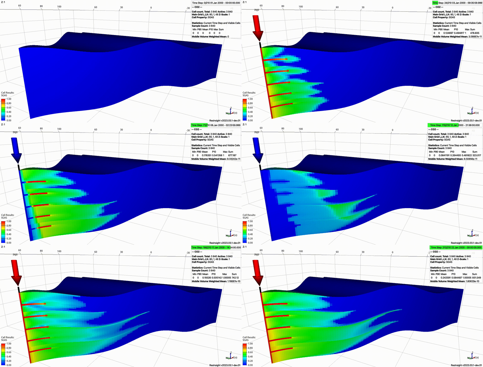
The execution time was c.a. 20 seconds and the following is an animation using ResInsight to visualize the gas saturation:

Simulation results of the gas saturation.

CCUS (machine learning)

See this folder for an example of how to use pyopmnearwell to generate data for different input parameters (e.g., injection rates) and read the data (e.g., production volumes). An additional example can be found in the data_generation folder. These examples could be used as a starting point for the ones interested in ML.

Publications

For the simulation results published in this paper about the impact of intermittency on salt precipitation during CO2 injection, see/run these configuration files.

For a study where pyopmnearwell is used to generated a machine-learned near-well model, click here.