Examples
For additional examples demonstrating the applicability of pycopm, see the tests.
ResInsight and plopm are used for the visualization of the results.
Note
There are binary packages for Linux and Windows to install Resinsight, see the ResInsight Documentation. For macOS users, you could try to install it using brew by executing:
brew install cssr-tools/opm/resinsight
Then, you should be able to open resinsight by typing in the terminal resinsight. If you have issues installing ResInsight, ParaView can be also used. However, you need to add the flag --enable-vtk-output=true to OPM Flow.
Via configuration files
The examples folder contains configuration files to perform HM studies in drogon and norne using ERT. For example, by executing inside the example folder for drogon:
# From inside the main pycopm folder
cd examples/configurations/drogon
pycopm -i input.toml -o drogon_coarser
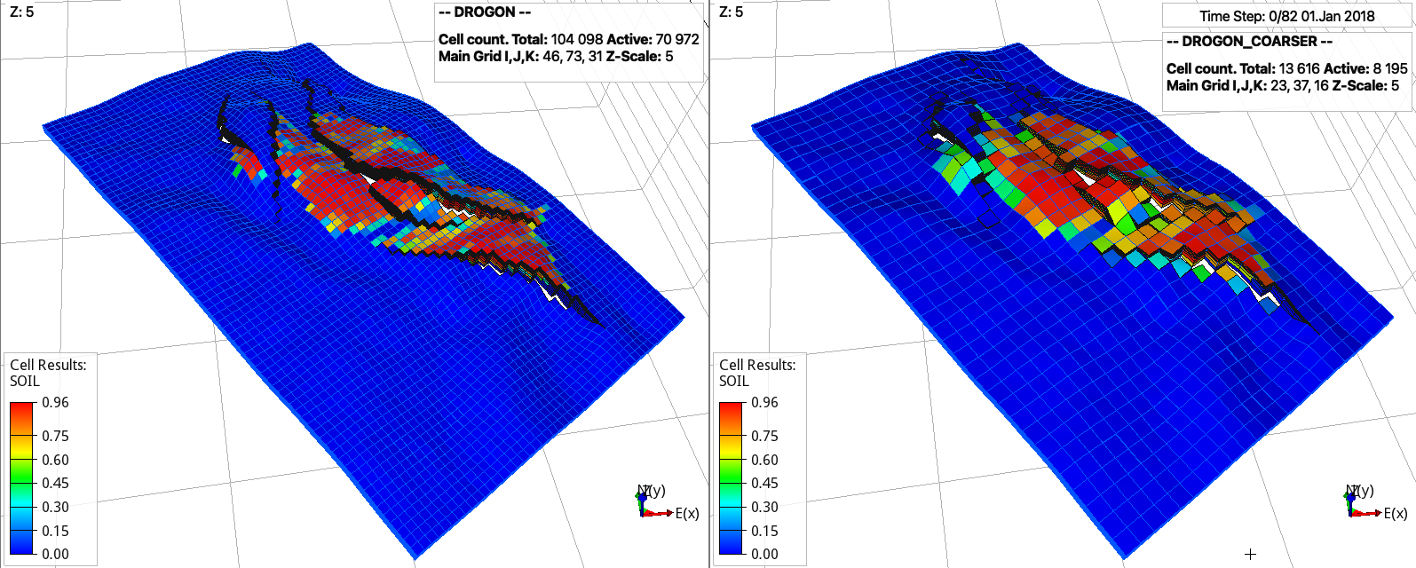
The following are the drogon model from opm-tests and coarsened model generated using pycopm using ResInsight for the visualization:
Note
For Drogon, a scored is printed after the run to compared the error to the results available at https://webviz-subsurface-example.azurewebsites.net/history-match. While input.toml only runs one HM iteration with two ensemble members that is used in testing pycopm, hm.toml runs a history matching with a better score (i.e., less error compare to the observation data). This configuration file is also an example of how to use mpi to run Flow built from source (set the flow path to your flow location; if you do not have mpi, you can remove it and still run the example).
Via OPM Flow decks
The current development of pycopm focuses on creating tailored models (grid refinement, grid coarsening, submodels, and transformations) by using input decks. While in the Hello world example these four different options are demonstrated, for the latter examples the focus is on the grid coarsening functionality, and the SPE10 also shows the submodel functionality.
Hello world
For the HELLO_WORLD.DATA deck, by executing:
# From inside the main pycopm folder
cd examples/decks
pycopm -i HELLO_WORLD.DATA -c 5,5,1 -m all -o output
Note
If the folder to flow is not added to your path, then pass the full path to the flow executable using the flag -f /path/to/flow.
Using ResInsight, then we can visualize the generated files in the output folder:
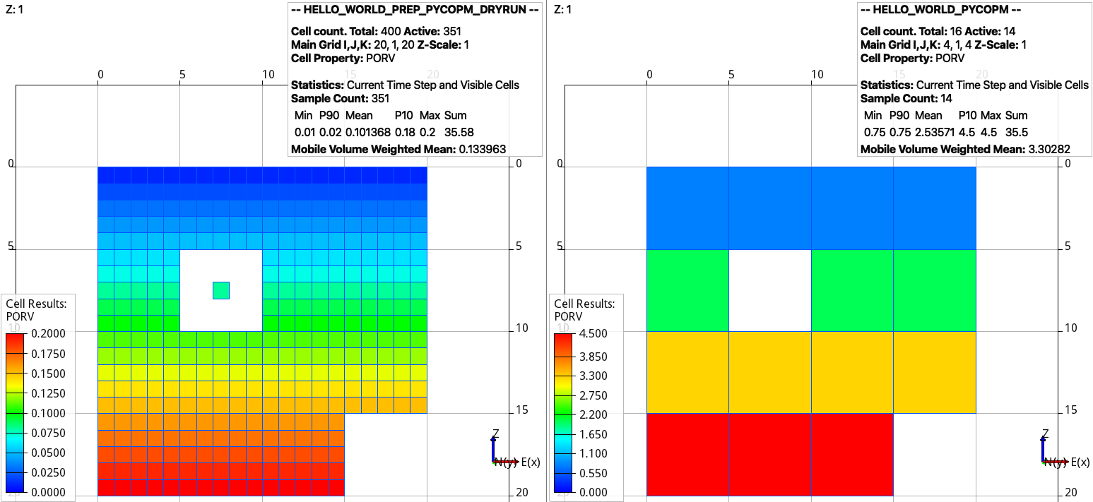
Dry run from the input cloned deck (left) and (right) coarsened model. Adding the flag -p 1 adds the remove pore volume to the neighbouring cells.
As mentioned above, if you do not have ResInsight, then to visualize the results in ParaView run
flow HELLO_WORLD.DATA --enable-vtk-output=true
flow HELLO_WORLD_PYCOPM.DATA --enable-vtk-output=true
To make active the coarsened cell where there is only one active cell, this can be achieved by:
pycopm -i HELLO_WORLD.DATA -c 5,5,1 -m all -a max
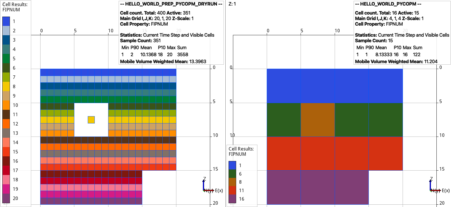
Dry run from the input cloned deck (left) and (right) coarsened model. The region numbers by default are given by the mode, e.g., use the flag -n max to keep the maximum integer.
As described in the theory, pycopm can be not only used for grid coarsening, but also to apply grid refinements, submodels, and transformations. Then, with the following commands first we substract a submodel around the isolated grid cell proyecting the outside pore volume on the boundaries, after we apply a grid refinement on the cells in the middle x and y location, and finally we rotate the model 45 degrees.
pycopm -i HELLO_WORLD.DATA -v 'xypolygon [4,8.5] [4,16.5] [11.5,16.5] [11.5,8.5]' -p 1 -m all
pycopm -i HELLO_WORLD_PYCOPM.DATA -rx 0,0,0,2,0,0,0 -ry 0,0,0,2,0,0,0 -m all
pycopm -i HELLO_WORLD_PYCOPM_PYCOPM.DATA -d 'rotatexy 45' -m all
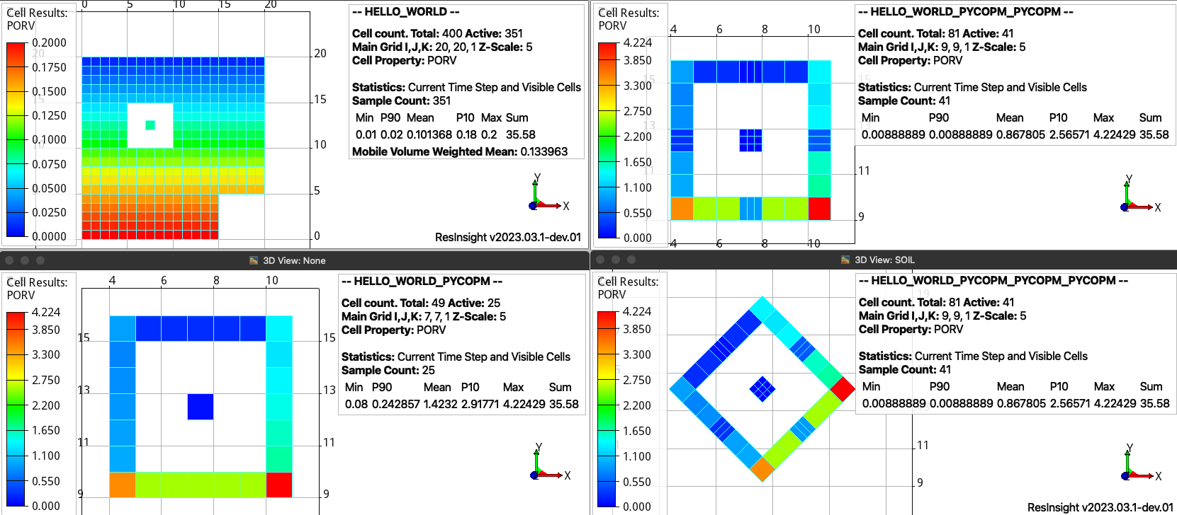
Extracted region with the projected pore volumes (bottom left), refinement around the center cells (top right), and rotation (bottom right). The text in the legends highlight that the pore volume is conserved (35.58) and the number of active cells is reduced from 351 to 25 in the submodel and after increased to 41 due to the grid refinement.
Note
To write the cell values for the SOLUTION section instead of using the EQUIL keyword, this can be achieved by the flag -explicit 1; the only requirement is that the EQUIL keyword needs to be in the main input DATA file and no via INCLUDE files.
Smeaheia
By downloading the Smeaheia simulation model (dataset part Simulation models), then:
# From the download folders
cd Simulation_Models/data
pycopm -c 5,4,3 -a min -m all -i Statoil_Feasibility_sim_model_with_depletion_KROSS_INJ_SECTOR_20.DATA -o .
will generate a coarser model five times in the x direction, four in the y direction, and three in the z direction, where the coarse cell is made inactive if at least one cell is inactive (-a min).
We use our plopm friend to generate PNG figures:
Tip
You can install plopm by executing in the terminal:
pip install git+https://github.com/cssr-tools/plopm.git
plopm -i 'STATOIL_FEASIBILITY_SIM_MODEL_WITH_DEPLETION_KROSS_INJ_SECTOR_20_PREP_PYCOPM_DRYRUN STATOIL_FEASIBILITY_SIM_MODEL_WITH_DEPLETION_KROSS_INJ_SECTOR_20_PYCOPM' -s ,,0 -v poro -subfigs 1,2 -save smeaheia -t 'Smeaheia Coarsened Smeaheia' -delax 1 -xunits km -xformat .0f -yunits km -yformat .0f -d 5,4.5 -suptitle 0 -c cet_rainbow_bgyrm_35_85_c69 -cbsfax 0.2,0.95,0.6,0.02 -cformat .2f
Top view of porosity values for the (left) original and (right) coarsened model (note that we also apply the coarsening on the z direction).
Drogon
Note
In the current implementation of the pycopm tool, the handling of properties that requires definitions of i,j,k indices (e.g., FAULTS, WELLSPECS) are assumed to be defined in the main .DATA deck. Then, in order to use pycopm for simulation models where these properties are define via include files, replace those includes in the .DATA deck with the actual content of the include files. Here are some relevant keywords per deck section that need to be in the main input deck and not via include files:
SECTION GRID: MAPAXES, FAULTS, MULTREGT (other keywords like MULTZ, NTG, or definitions/operations for perms and poro can be in included files since permx, permy, permz, poro, porv, multx, multy, multz are read from the .INIT file)
SECTION PROPS: EQUALS, COPY, ADD, and MULTIPLY since this involve i,j,k indices and are applied to properties such as saturation functions parameters that are still given in the same input format in the generated deck. In addition, SWATINIT if used in the deck, is read from the .INIT file and output for the modified deck in a new file, then one might need to give the right include path to this special case.
SECTION SCHEDULE: All keywords in this section must be in the input deck and no via include viles.
Following the note above, then by downloading the DROGON model, adding the MAPAXES to the deck, replacing the lines in DROGON_HIST.DATA for the FAULTS (L127-128) and SCHEDULE (L242-243) with the actual content of those include files, then by executing:
pycopm -i DROGON_HIST.DATA -c 1,1,3 -p 1 -q 1 -l C1
pycopm -i DROGON_HIST_PYCOPM.DATA -c 1,3,1 -p 1 -q 1 -j 2.5 -l C2 -m all
this would generate the following coarsened model:
Note that the total pore volume is conserved for the coarsened model (right). The properties of the standard model (left) can be visualized using the DROGON_HIST_PREP_PYCOPM_DRYRUN generated files.
Here, we first coarse in the z direction, which reduces the number of cells from 31 to 11, and after we coarse in the y direction. After trial and error, the jump (-j) is set to 2.5 to avoid generated connections across the faults. For geological models with a lot of inactive cells and faults, this divide and conquer apporach is recommended, i.e., coarsening first in the z direction and after coarsening in the x and y directions. Also, we add labels (-l) C1 and C2 to differentiate between the coarse include files. In addition, we use the flags -p 1 -q 1 to add the remove pore volume to the closest coarser cells and to redistribute the pore volume in the locations with gas and oil, this results in the coarsened model having the same total pore volume, field gas in place, and practically same oil and water in place as the input model.
Note
Add to the generated deck the removed include files in the grid section related to the region operations (e.g., ../include/grid/drogon.multregt for this case).
Now, we also show a two times coarsened model in all directions (referring to the previous comment about divide and conquer, for the Drogon model it seems still ok to do a two times coarsening in one go):
pycopm -i DROGON_HIST.DATA -c 2,2,2 -p 1 -q 1 -j 4 -w DROGON_2TIMES_COARSER -m all
Here, we use the -w flag to give a specific name to the generated coarsened deck, as well as using a higher value of -j to avoid generated connections across the faults.
Tip
To use a different approach from the default ones (see the theory) to coarse one of the properties (e.g., permeabilities), this can be achieve by the -s flag, e.g., -s pvmean to coarse the permeabilities using a pv-weighted mean. In addition, one could add a different label -l pvweightedperms to identify the generated .INC files with the permeabilities, and rename these files in order to be used in the coarserned model with the rest of the properties using the default aproaches or a combination of them (e.g., -s max -l maxpermz and keep the maximum values of permz).
If we run these three models using OPM Flow:
flow DROGON_HIST.DATA
flow DROGON_HIST_PYCOPM_PYCOPM
flow DROGON_2TIMES_COARSER
then we can compare the summary vectors. To this end, we use our good old friend plopm:
plopm -i 'DROGON_HIST DROGON_HIST_PYCOPM_PYCOPM DROGON_2TIMES_COARSER' -v 'FOIP,FOPR,TCPU' -tunits y -f 14 -subfigs 2,2 -delax 1 -loc empty,empty,empty,center -d 10,5 -xformat '.1f' -xlnum 6 -ylabel 'sm$^3$ sm$^3$/day seconds' -t 'Field oil in place Field oil production rate Simulation time' -labels 'DROGON DROGON 3XZ COARSER DROGON 2XYZ COARSER' -save drogon_pycopm_comparison -yformat '.2e,.0f,.0f'
Note that the coarsened models have the same initial field oil in place as the input model. It seems the coarsened properties (e.g., permeabilities) are good initial inputs to use in a history matching framework (e.g., to history match saturation function parameters), and the lower simulation time for the coarsened models allow for more ensemble members and more iterations.
We can also make a nice GIF by executing:
plopm -v sgas -subfigs 1,3 -i 'DROGON_HIST DROGON_HIST_PYCOPM_PYCOPM DROGON_2TIMES_COARSER' -d 16,10.5 -m gif -dpi 300 -t "DROGON DROGON 3XZ COARSER DROGON 2XYZ COARSER" -f 16 -interval 2000 -loop 1 -cformat .2f -cbsfax 0.30,0.01,0.4,0.02 -s ,,1 -rotate -30 -xunits km -yunits km -xformat .0f -yformat .0f -c cet_rainbow_bgyrm_35_85_c69 -delax 1 -r 0:3
Top view of the Drogon and the two coarsened models
Norne
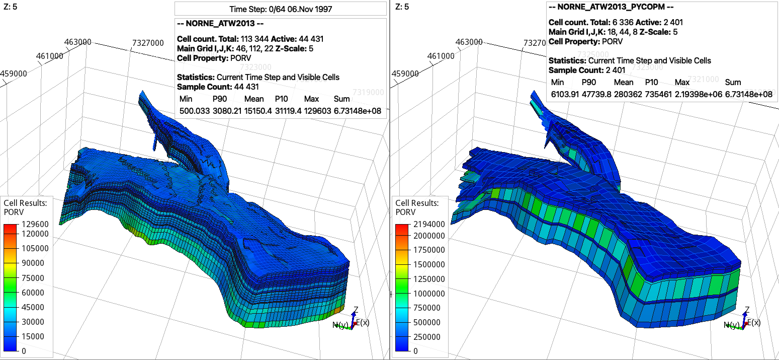
By downloading the Norne model (and replacing the needed include files as described in the previous example, specially the include file ./INCLUDE/BC0407_HIST01122006.SCH at the end of NORNE_ATW2013.DATA to run the example without errors), then here we create a coarsened model by removing certain pilars in order to keep the main features of the geological model:
pycopm -i NORNE_ATW2013.DATA -s pvmean -x 0,2,0,2,2,0,2,0,2,0,2,0,2,2,0,2,0,2,2,0,2,0,2,2,0,2,0,2,2,0,2,0,2,0,2,0,2,2,0,2,2,0,2,2,2,2,0 -y 0,2,0,2,2,0,2,0,2,2,0,2,0,2,2,0,2,0,2,2,0,2,0,2,2,0,2,0,2,2,0,2,0,2,2,0,2,0,2,2,0,2,0,2,2,0,2,0,2,2,0,2,0,2,2,0,2,0,2,2,0,2,0,2,0,2,0,2,2,0,2,0,2,2,0,2,0,2,2,0,2,0,2,2,0,2,0,2,0,2,0,2,0,2,0,2,0,2,0,2,0,2,0,2,2,2,2,2,2,2,2,2,0 -z 0,0,2,0,0,2,2,2,2,2,0,2,2,2,2,2,0,0,2,0,2,2,0 -a min -p 1 -q 1 -m all
this would generate the following coarsened model:
SPE10
By downloading the SPE10_MODEL2 model, then:
pycopm -i SPE10_MODEL2.DATA -s pvmean -c 4,8,2 -m all
generates a coarsened model from ca. 1 million cells to ca. 20 thousands cells.
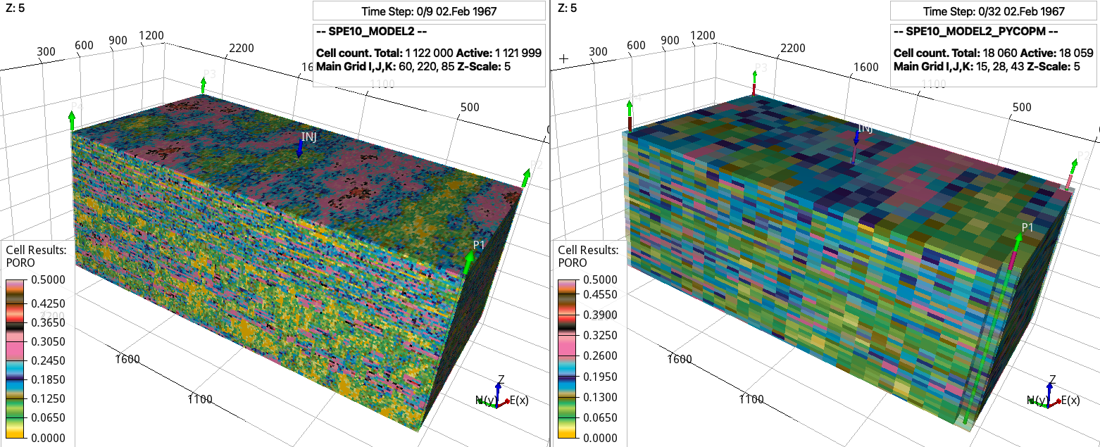
Porosity values for the (left) original and (right) coarsed SPE10 model.
To generate a submodel from the coarsened model around the injector ‘INJ’, this can be achieved by executing:
pycopm -i SPE10_MODEL2_PYCOPM.DATA -p 1 -v 'INJ diamondxy 5' -m all -w vicinity -l sub -m all
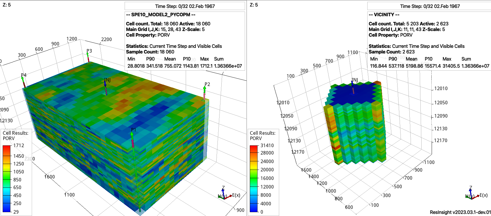
Pore volume values for the (left) coarsened and (right) vicinity around the well INJ in the SPE10 model.
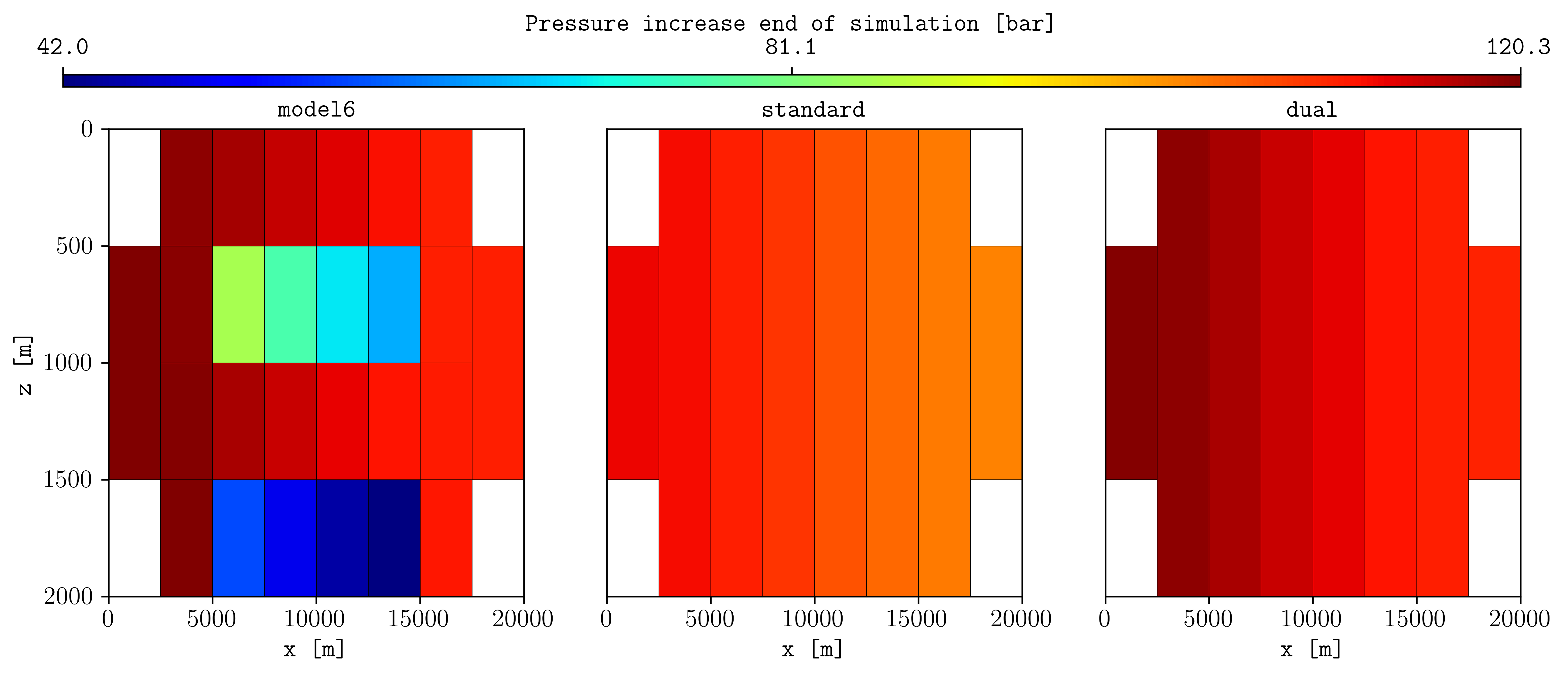
Dual coarsening
The flag -dual allows to perform a coarsening by differentiating between net and non-net cells, resulting in two coarsened grids. For example, using the MODEL6.DATA:
pycopm -i MODEL6.DATA -z 1:4 -w STANDARD -l S -t 2 -a max
pycopm -i MODEL6.DATA -z 1:4 -w DUAL -dual 'poro <= 0.1' -l D -t 2 -a max
flow MODEL6.DATA
flow STANDARD.DATA
flow DUAL.DATA
plopm -i 'MODEL6 STANDARD DUAL' -v 'pressure - 0pressure' -subfigs 1,3 -delax 1 -cbsfax 0.1,0.95,0.8,0.02 -d 12,4  -suptitle 0 -z 0 -clabel 'Pressure increase end of simulation [bar]' -grid 'black,1e-2'
This results in the following figure, where the pressure on the most right cell compares better using the dual coarsening than the standard:
Graphical abstract
Here we describe how to generate the geological model ilustrations in the graphical abstract. These five ilustrations are generated from the DROGON_HIST.DATA model, and the visualization is achieve using ResInsight.
Top figure: By running the DROGON_HIST.DATA using opm flow and visaluazing the static property pore volume.
Coarsenings: This corresponds to the generated DROGON_HIST_PYCOPM_PYCOPM.DATA deck in Drogon.
Submodels: pycopm -i DROGON_HIST.DATA -v ‘xypolygon [463739,5931508] [464872,5932123] [464401,5932862] [463284,5932209] [463739,5931508]’ -w SUBMODELS -m all
Refinements: pycopm -i SUBMODELS.DATA -g 2,2,2 -w REFINEMENTS -m all
Transformations: pycopm -i DROGON_HIST.DATA -d ‘rotatexy 45’ -w TRANSFORMATIONS -m all
Note that for ResInsight to show the wells, one needs to run the decks (e.g., flow REFINEMENTS.DATA).