Theory

Here insight about the pycopm methods regarding grid coarsening, grid refinement, submodels, and transformations is given.

Grid coarsening

The coarsening approach implemented in pycopm is based on industry standard grid formats which is preserved during coarsening. This allows for direct application in standard reservoir simulators. In coarsening accuracy is traded for speed. This is often appropriate, but care must be taken to assure that the coarse solution preserve the key properties of the model. The Lie 2019 textbook gives an excellent introduction to grid coarsening and upscaling geological properties, and the methods implemented in pycopm follow similar techniques.

Corner-point grids are commonly use in subsurface simulations, due to its flexibility to handle complex geometries such as faults. The grid is defined by vertical pillars and horizontal lines connecting the pillars, resulting in cells that can have up to six faces (hexahedrons), but also these grids allow to define connections between non-neighboring cells (NNC). A special case of corner-point grids are Cartesian regular grids. These grids also feature inactive cells, which are cells with zero pore volume and no connected to the active cells.

We define the grid coarsening operator \(\Xi_{xyz}^C\), which creates from an input grid \(\Omega\) a coarser grid \(\Omega^*\) (we adopt the notation * for coarser quantities, while \({}^C\) in the coarsening operator emphasize the different approaches for the cell clustering) by removing vertical pillars and horizontal lines:

\[\Xi_{xyz}^C(\Omega)\rightarrow\Omega^*\]

To give flexibility in the coarsening, the cell clustering can be given as x, y, and z arrays to define the pillars/lines to be removed. One natural question is how to handle the inactive cells in a cluster, and for this, three options to define the coarser cells are implemented: min, max, and mode (mode is the default, i.e., the coarser cells is active if the number of active cells is the most common value in the cluster). Figure 1 shows a simple 2D corner-point grid with different coarsening using min, max, and mode.

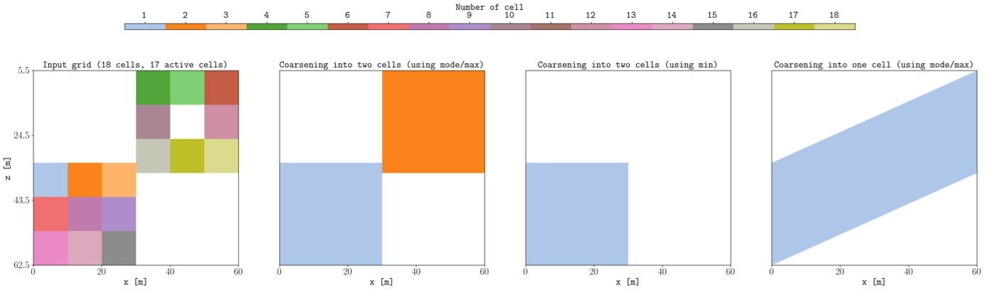
Figure 1: Example of coarser models from a grid with 18 cells, where the cell #11 is inactive. One example where the max option could be useful is for models where there are a lot of inactive cells in the z direction, while the min option could be useful for models applying coarsening in the xy plane, since using min results in coarser models that do not generate new connections across inactive cells.

For upscaling geophysical properties, naturally, the pore volume in a coarser cell \(\Phi_{i^*,j^*,k^*}^*\) (\(i^*\), \(j^*\), and \(k^*\) referring to the cell coarse indices in the x, y, and z direction respectively) are equal to the sum of pore volume from the corresponding cells \(\Phi_{i,j,k}\) in the input model, which are part of the cluster \(\mathbb{C}_{i^*,j^*,k^*}\):

\[\Phi_{i^*,j^*,k^*}^* = \sum_{(i,j,k)\in\mathbb{C}_{i^*,j^*,k^*}}\Phi_{i,j,k}\]

For example, in Figure 1 when coarsening into two cells using mode/max resulted in two coarse cells, where:

\[\mathbb{C}_{1^*,1^*,1^*}=\{ (1,1,1),(2,1,1),(3,1,1),(1,1,2),(2,1,2),(3,1,2),(1,1,3),(2,1,3),(3,1,3) \}.\]

From this definition, the porosity in the coarse model \(\phi_{i^*,j^*,k^*}^*\) can be simply computed by:

\[\phi_{i^*,j^*,k^*}^* = \frac{\Phi_{i^*,j^*,k^*}^*}{\mathbb{V}_{i^*,j^*,k^*}^*}\]

where \(\mathbb{V}_{i^*,j^*,k^*}^*\) is the geometric volume of the coarser cell.

For the rock permeability, there are different upscaling methods (e.g., arithmetic or harmonic average) that are case dependent and perform different, see the Lie 2019 textbook for comparison of these methods. In pycopm, by default the permeability in the x and y directions are computed using the arithmetic average, while the permeability in the z direction by the harmonic average. As additional options, the permeabilities in the coarser cells \(\mathbb{K}_{i^*,j^*,k^*}^*\) can be set to equal the min, max, mean, or pv-weighted mean (pvmean) values from the permeabilities in the corresponding cluster \(\mathbb{K}_{i,j,k}\). For example, using the max for permeabilities could be useful for history matching studies, where the parameters to history match are saturation functions (relative permeabilities and capillary pressure).

The above line mentions the initial application to develop pycopm (coarsening to history match saturation functions), as such there are no upscaling methods implemented in pycopm for saturation functions. In a geological model, it is common to define different regions (referred as satnum) to assign different saturation function tables. Then, if a cluster \(\mathbb{C}_{i^*,j^*,k^*}\) involves different values for satnum, the mode (the most frequent value) is used to assign the value in the coarser cell (this is also used to assign additional discrete coarser values such as fluid-in-place regions (fipnum)).

For grids with large number of non-neighboring connections (faults) and inactive cells, then a better approach is to upscale transmisibilities. A drawback of upscaling transmissibilities is that permeabilities cannot be used in history matching, but instead, transmissibilities multipliers, which increases the number of parameters to history match and might break history match workflows where different permeability fields are generated from spatial correlations. To this end, two approaches to upscale transmissibilities are implemented in pycopm. The former computes the coarser transmissibility

\[\scriptsize\mathbb{T}_{i^*,j^*,k^*}^*=\left[ T_{i^*,j^*,k^*\rightarrow i^*+1,j^*,k^*}^*,T_{i^*-1,j^*,k^*\rightarrow i^*,j^*,k^*}^*,T_{i^*,j^*,k^*\rightarrow i^*,j^*+1,k^*}^*,T_{i^*,j^*-1,k^*\rightarrow i^*,j^*,k^*}^*,T_{i^*,j^*,k^*\rightarrow i^*,j^*,k^*+1}^*,T_{i^*,j^*,k^*-1\rightarrow i^*,j^*,k^*}^* \right]\]

using the armonic averaging along the transsmissibility direction and summing over these values over the cell coarser face. For example, for the transmissibility in the z+ direction:

\[T_{i^*,j^*,k^*\rightarrow i^*,j^*,k^*+1}^*=\sum_{(i,j)\in\mathbb{C}_{i^*,j^*,k^*}}\left( \sum_{(i,j,k)\rightarrow(i,j,k+1)\in\mathbb{C}_{i^*,j^*,k^*}} \frac{1}{T_{i,j,k\rightarrow i,j,k+1}} \right)^{-1}\]

For cases where the coarsening is only along one direction (e.g., the z direction), the second method sets the transmissibility on the coarse cell faces in that direction equal to the overlapping cell face values in the corresponding cluster (instead of computing the armonic average). For input models with a large number of inactive cells, this approach has resulted in better results with respect to the input model simulations than using the armonic average. For both approaches, the transmissibilities are scaled with the ratio of the cell face effective areas (input model) to the coarse cell area. For non-neighbouring connections, this approach is also implemented, i.e., the non-neighbouring connections in the coarser model sum the values from the non-neighbouring connections in the input model, which is important in order to honor the pressure connections along open faults communicating different formations.

Grid refinement

The grid refinement is achieved by adding vertical pillars and horizontal lines in the grid from the input model. The refinement can be defined globally in any direction (i, j, or k), as well as localized in defined grid indices. Properties such as porosity, permeabilities, and region numbers are set to the same value in the corresponding finner cells inside the unrefined cell. Model properties defined by i,j,k locations such as wells, faults, and boundary conditions are mapped to the new range of refined indices (i.e., adding additional entries to the generated deck).

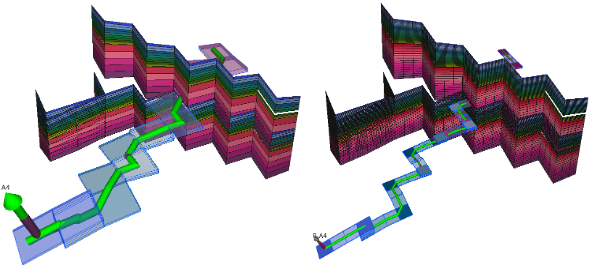
Figure 2: Faults and well in MODEL3.DATA (left) and after grid refinement “-g 2,2,2” (right).

Submodels

The generation of a submodel, i.e., a selected region in the input model, makes possible to lower the number of active cells and focus on an area of interest in the input model. This results in smaller size of the input files, and faster simulations using OPM Flow. The submodel can be defined by properties matching a value, e.g., all cells with fipnum equal to 1, or by a polygon given the xy locations in meters. Model properties defined by i,j,k locations such as wells and faults are shifted to their corresponding values. If the wells/faults are not inside the extracted submodel, then these are not written to the generated deck.

Regarding the boundary conditions in the extracted model with respect to the pore volume outisde the submodel, four options are provided by pycopm:

1. no correction for the pore volume

2. adding the pore volume in each cell on the submodel boundary by summing all cell pore volumes in their corresponding i and j directions. If there is pore volume in the outside corners, this is equally distributed among the boundary cells in the two corresponding sides.

3. distributing the pore volume equally among the boundary cells in the submodel.

4. distributing the pore volume equally among all cells in the submodel

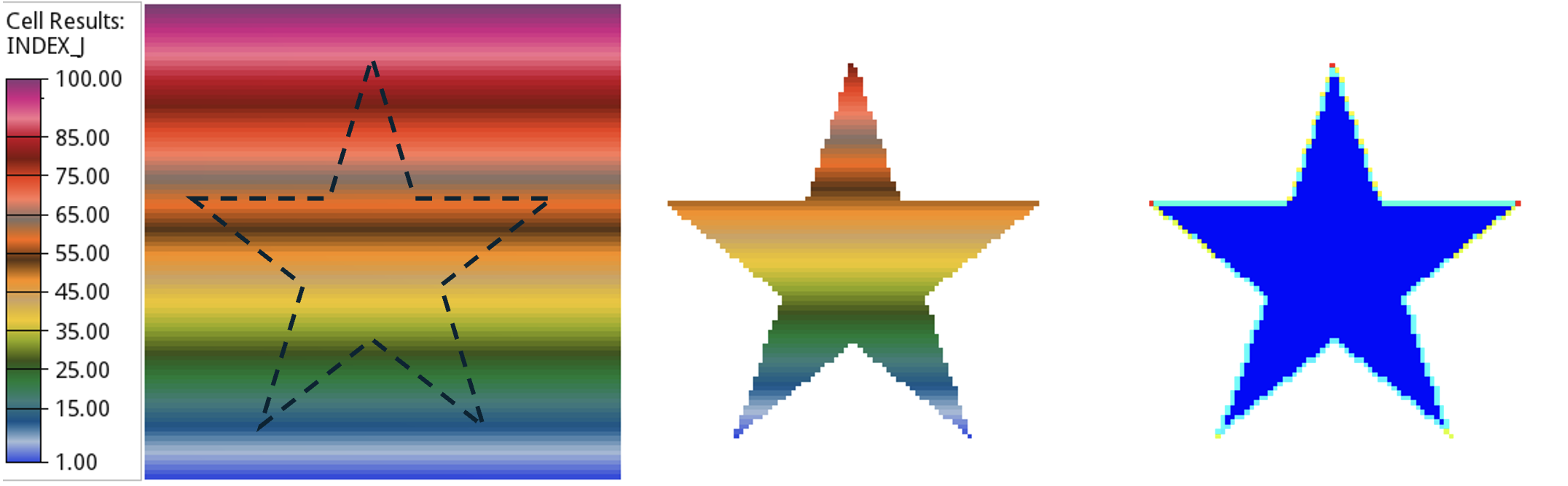
Figure 3: The shape to extract the sudmodel corresponds to “-v ‘xypolygon [50,90] [60,60] [90,60] [65,40] [75,10] [50,30] [25,10] [35,40] [10,60] [40,60] [50,90]’”. The j indices for the cells have been accordingly shifted in the extracted model, and the right figure shows the projected pore volume on the boundary.

In addition, it is possible to extract submodels around wells, with three different options for the neighbourhood: box, diamond, and diamondxy. The box option allows to define the intervals to extract the cells, while the diamond and diamondxy results in fewer cells since the cells in the corners are trimmed.

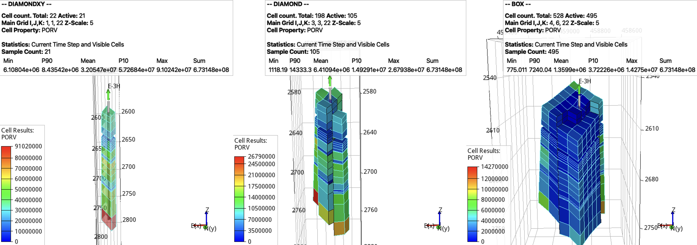
Figure 4: The submodel in norne by executing “-v ‘E-3H diamondxy 0’ -p 1”, “-v ‘E-3H diamond 1’ -p 1”, and “-v ‘E-3H box [-1,2] [-2,3] [-1,1]’ -p 1” respectively.

Transformations

Affine transformations are widely used in diverse applications since they preserve points, straight lines, and planes. In the field of reservoir management, there are large uncertainties in the characterization of geological formations (reservoirs are typically located several kilometers below the surface). Once a reservoir model is created, over time additional information from field measurements (e.g., seismic data, addiitonal wells, well’s pressures, production rates) can indicate a different model characterization. This is when having tools like pycopm can be handy, i.e., to apply translations of the grid (e.g., a different depth which impacts the pressure), scaling (e.g., to ease comparison between models made by different groups which missmatch in the thickness of layers), and rotations (e.g., to align grids betweens two different models).

Figure 5: Extracted shape in Figure 3 after a rotation “-d ‘rotatexy 45’” (left) and scaling “-d ‘scale [1,0.25,1]’” (right).