Reading CSV files

Read time-series and spatial-map CSV files, compare benchmark submissions, and combine CSV data with OPM Flow output.

CSV column syntax

Use plopm -cc to identify the columns in each CSV input. Column indices start at 1:

• Use time,value for a time series, for example 1,3.

• Use x,y,value for a spatial map, for example 1,2,5.

• Separate specifications for multiple inputs with semicolons.

• Leave one specification empty when the corresponding input is an OPM Flow result rather than a CSV file.

Compare simulation and reporting grids

Compare liquid-phase CO2 mass fraction on the OPM Flow simulation grid with the same quantity from the regular benchmark reporting grid:

plopm -v xco2l -i 'r1_Cart_10m/R1_CART_10M r1_Cart_10m/spe11b_spatial_map_500y' -cc ';1,2,5' -sg 2,1 -rdl 1 -r 100 -fs 10,3 -st 0 -t 'Simulation grid  Reporting grid' -cbp 0.35,0.97,0.3,0.02 -yu km -xu km -yf .1f -xf .1f -cbn 5 -xnt 8 -cbf .2f

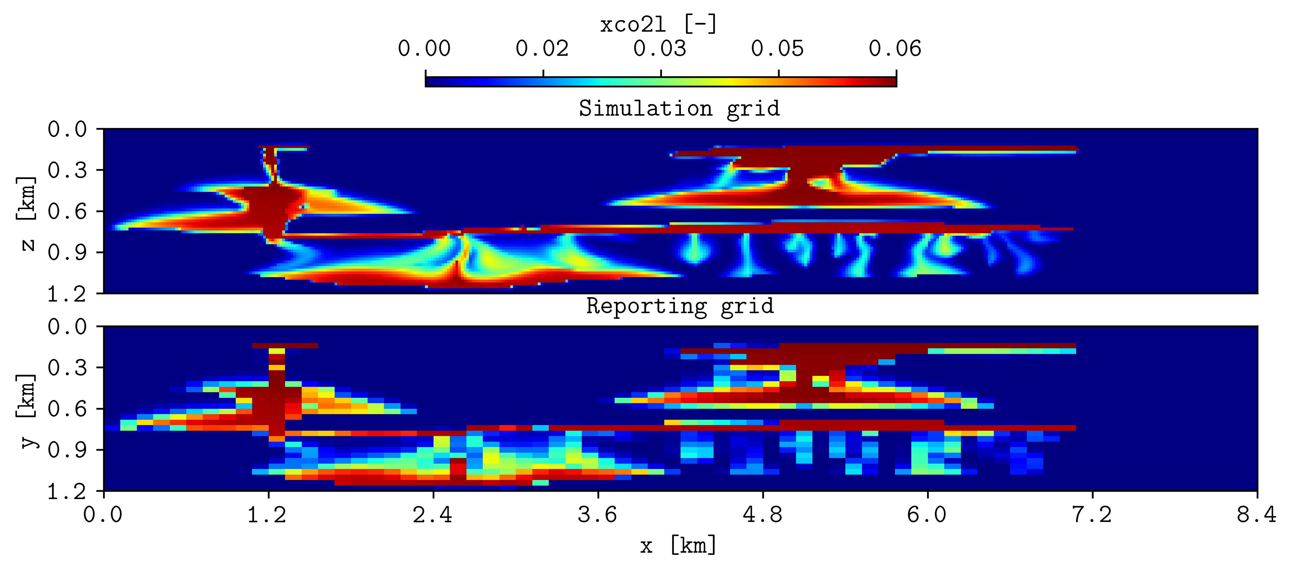
Liquid-phase CO2 mass fraction from the OPM Flow simulation grid and the SPE11B reporting-grid CSV file at 500 years.

The first column specification is empty because the first input is an OPM Flow case. The second input uses columns 1, 2, and 5 for x, y, and the plotted value.

Compare CSV and OPM summary data

Compare a pressure time series from a CSV file with the corresponding OPM Flow summary vector:

plopm -i 'r1_Cart_10m/spe11b_time_series r1_Cart_10m/R1_CART_10M' -v ',BWPR:256,1,5' -cc '1,3;' -sf '1e-5,1' -ls 'solid,dotted' -lw '4,4' -yl 'Sensor pressure [bar]' -llb 'From CSV file  From OPM Flow output file' -c 'r,k'

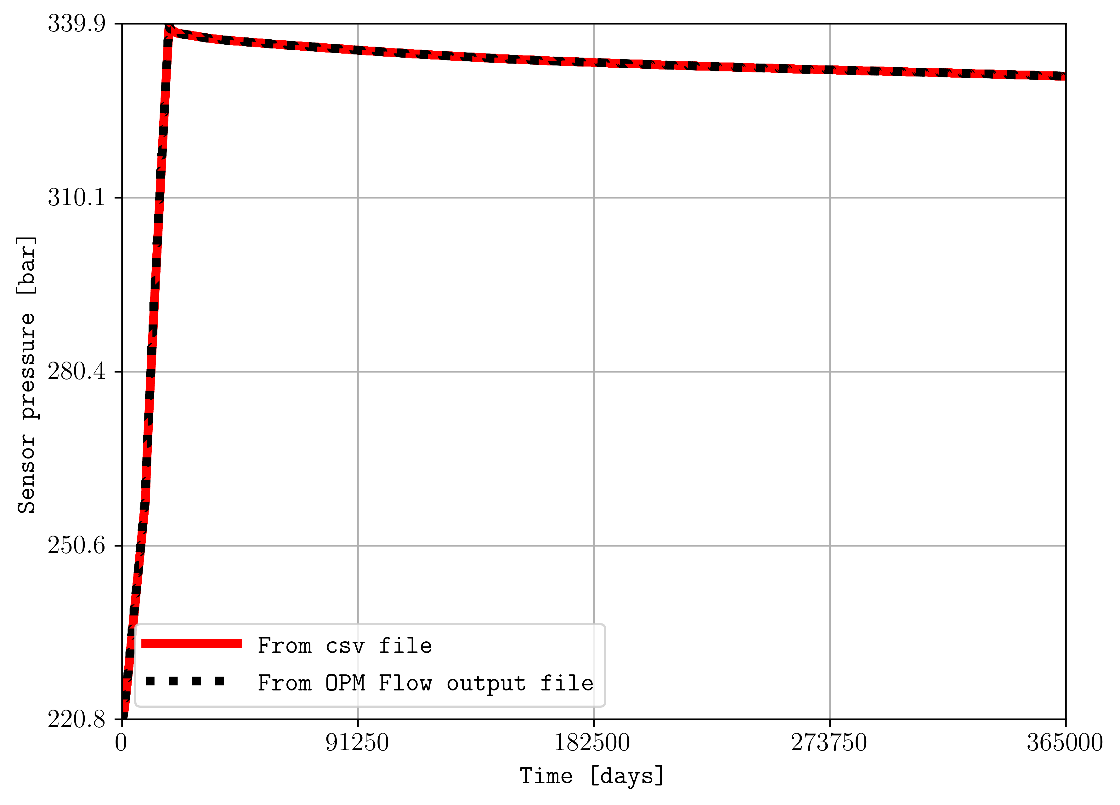
Sensor pressure read from the SPE11B time-series CSV file and directly from the OPM Flow summary output.

The empty first entry in plopm -v is a placeholder for the CSV input. The empty second entry in plopm -cc indicates that the second input is read as OPM Flow output. The scale factors convert the two sources to the same displayed unit.

Compare benchmark time series

After downloading the selected SPE11 benchmark submissions, compare the same CSV quantity from several participants and the pyopmspe11 simulation:

plopm -i 'opm1/spe11b_time_series opm2/spe11b_time_series opm3/spe11b_time_series opm4/spe11b_time_series r1_Cart_10m/spe11b_time_series' -cc '1,4;1,4;1,4;1,4;1,4' -tu y -x '[0,1000]' -yl 'dissA [kiloton]' -yf .1f -sf 1e-6 -c '#a8d8e3,#a8d8e3,#a8d8e3,#a8d8e3,#fc035a' -lw 5,5,5,5,5 -ls solid

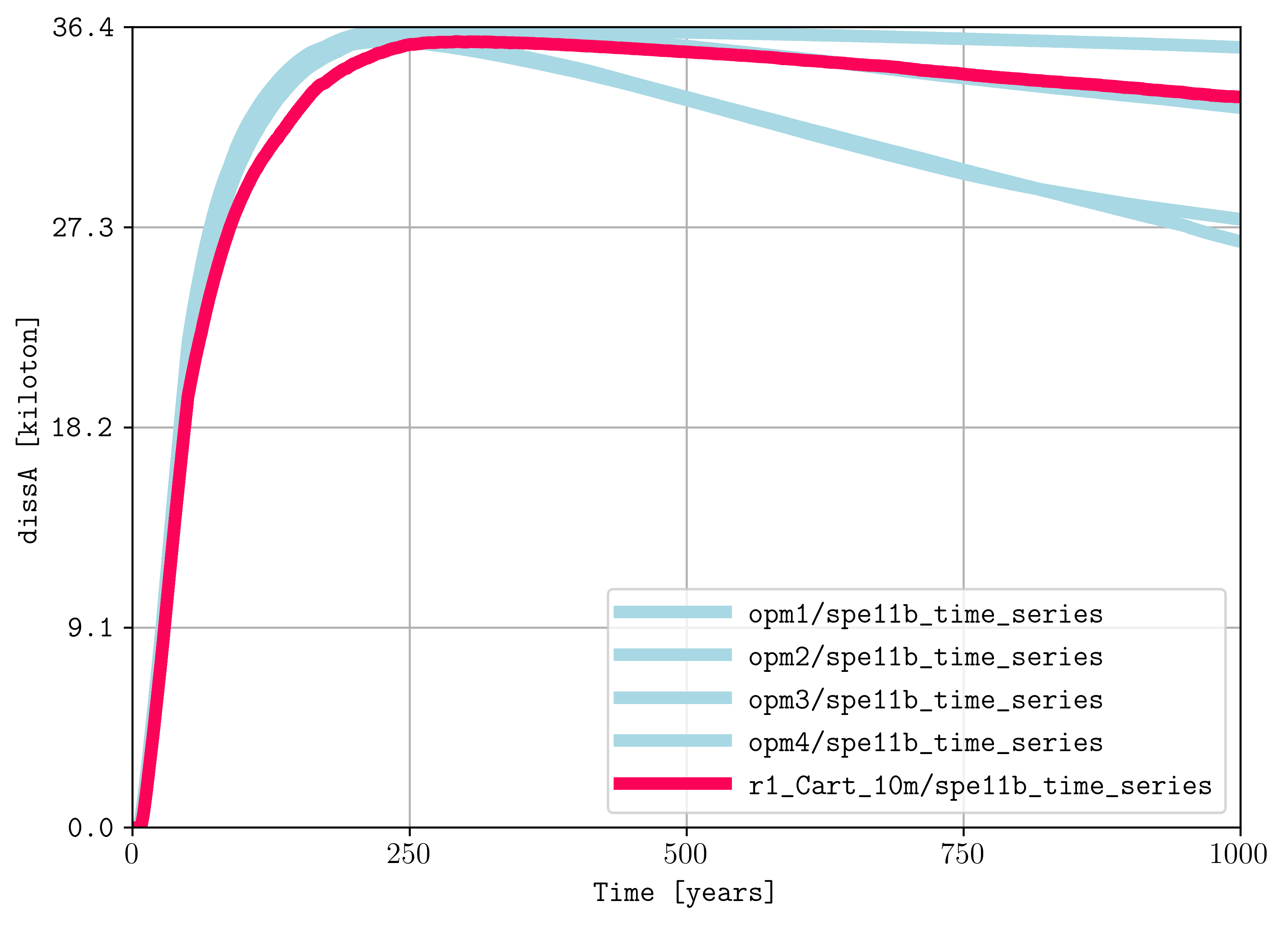
Dissolved CO2 mass in box A for several benchmark submissions and the pyopmspe11 simulation.

Each input uses columns 1 and 4. The scale factor converts kilograms to kilotonnes, and the color selection highlights the local simulation.

Compare benchmark spatial maps

Compare the same CSV spatial quantity from several benchmark submissions in a single subplot layout:

plopm -i 'opm1/spe11b_spatial_map_250y opm2/spe11b_spatial_map_250y opm3/spe11b_spatial_map_250y opm4/spe11b_spatial_map_250y r1_Cart_10m/spe11b_spatial_map_250y' -cc '1,2,5;1,2,5;1,2,5;1,2,5;1,2,5' -sg 3,2 -rdl 1 -st 0 -cbp 0.35,0.97,0.3,0.02 -yu km -xu km -yf .1f -xf .1f -cbn 5 -xnt 8 -cbf .2f -fs 14,4 -t 'opm1  opm2  opm3  opm4  my simulation' -cbl 'Time 250 years, CO$_2$ mass fraction (liquid phase) [-]' -c inferno

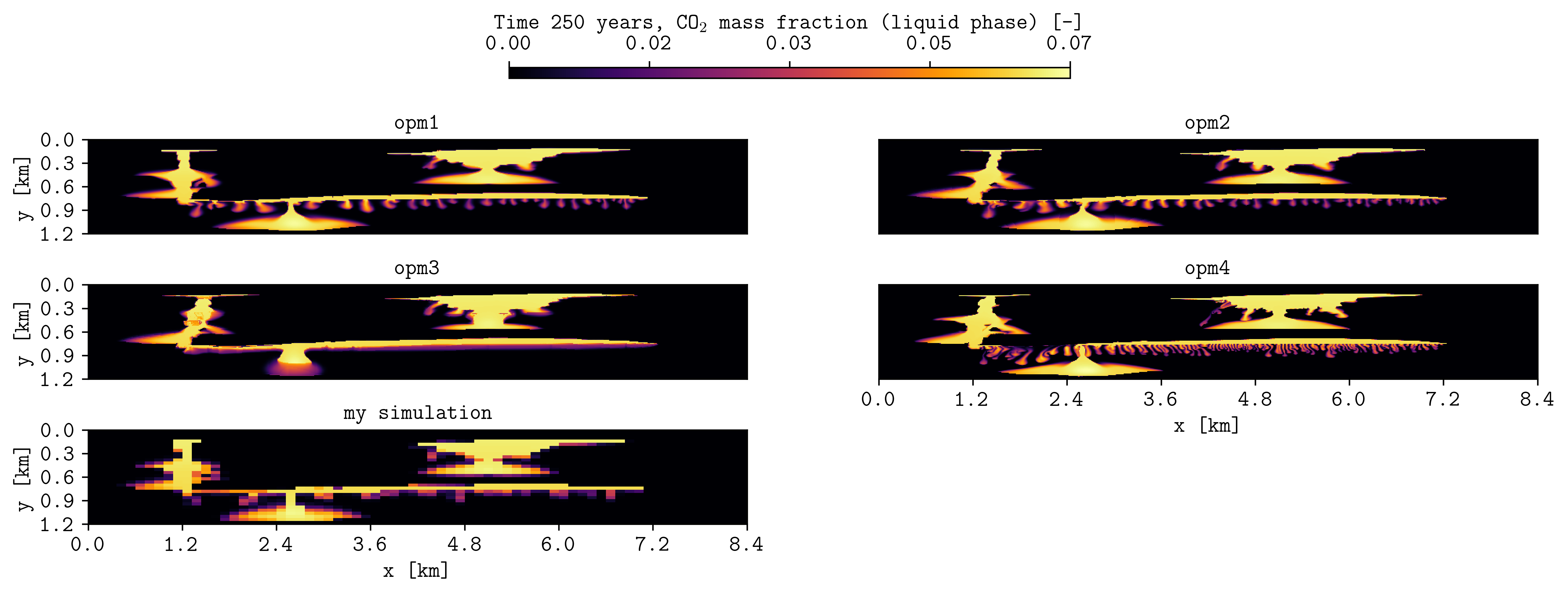
Liquid-phase CO2 mass fraction at 250 years for several benchmark submissions and the pyopmspe11 simulation.

All inputs use columns 1, 2, and 5 for x, y, and liquid-phase CO2 mass fraction. A global colorbar makes the maps directly comparable.

Create animations from CSV sequences

To create a GIF from a sequence of CSV spatial-map files, include PLOPM in the input filename where the time value changes. Select the required times with plopm -r and use -m gif. plopm replaces PLOPM with each selected time when reading the files.

Reproduce this example

Run the complete workflow from the repository root. The script downloads or prepares the required benchmark CSV inputs before generating the figures:

. ./tests/scripts/docs_reading_csvs.sh

View script

View raw script

Back to the examples gallery